Gauss’s Lemma is not a horrible combinatorial calculation

I’m not really sure why I’ve never seen this argument before, but it’s much cleaner and easier to digest than the arguments I’m used to that make Gauss’s Lemma look like it’s not part of algebra at all.

Definition. A polynomial with integer coefficients is primitive if its coefficients are relatively prime.

Lemma. (Gauss) The product of primitive polynomials is primitive.

Proof. Notice first that a polynomial is primitive iff no prime divides all its coefficients, iff it is not the zero polynomial (mod p) for any prime p.

Suppose two polynomials f and g are primitive. Then for each prime p neither f nor g is the zero element in . Since this ring is an integral domain, it follows that f g is not the zero element either. As this holds for all primes p, f g is primitive.

How to get GAP4 to describe a group

This is a command that’s tough to Google even if you know it exists.  To get GAP to describe a group with a common, human-readable name, you can use the StructureDescription command, as follows:

gap> StructureDescription(Group([(1,3), (1,2,3,4)]));

"D8"

gap> StructureDescription(Group([(1,3), (1,2,3)]));

"S3"

Documentation for theStructureDescription command is here.

1988 IMO Problem 6

Problem 6 of the 1988 International Math Olympiad reads:

Let a and b be positive integers such that a b + 1 divides .  Show that is the square of an integer.

There’s a writeup of a solution at the Art of Problem Solving wiki, but I found it incredibly sketchy and difficult to read and the article was locked, so here’s what’s hopefully an easier-to-read exposition of the same solution:

In other words, we’d like to show that any solution in positive integers to the equation has c a perfect square.

First, suppose we have a solution with a = b.  Then divides . Applying the Euclidean algorithm,

so we must have .  Since a is positive, we must have a=1.  In this case, so c = 1 which is a perfect square.  So we may assume in what follows that .

Fix a positive integer c for which the equation has solutions in the positive integers, and let (a, b, c) be such a solution with the minimum possible value of a.  Note that by symmetry we must have a < b, since otherwise (b, a, c) is a solution with a smaller first coordinate.

Rewrite the equation as

and notice that this says that b is a root of the quadratic equation

Let r denote the other root.  Then b + r = c a and .  It follows that is an integer, and that

So r < a.  This must mean that , as otherwise the solution (r, b, c) to the original equation would contradict the minimality of a.

Now

Since b + 1 is positive, we must have r + 1 positive as well.  Since r is an integer, we must have r = 0, so

or in other words .

 

The Poisson Summation Formula

There are various conventions for normalizing the Fourier transform. For the purposes of this post, let’s write

The Poisson Summation Formula concerns the sum

Where on Earth did that come from? Well, without regard to convergence issues, we have

So we see that we’re just transforming our function with respect to the kernel

Problematically, this doesn’t converge to a function. However, it does converge to a distribution. Let’s take a look at how it looks for a few values of n:

Figure: for N from 0 to 5.

As illustrated by the figure, the sequence is converging to a Dirac Comb, a periodic sequence of Dirac deltas.  From here the Poisson summation formula should be clear.  Alternatively, we could have started by (formally) working out the Fourier series for the Dirac comb, and we’d quickly arrive at the Poisson summation formula.

 

Elliptic integrals, I

This has tripped me up in the past, so let’s write it down.

Imagine we have an ellipse

Let’s say we have some parametrization (x(t), y(t)) of the ellipse and we want to convert it into a unit-speed parametrization. We can do this by composing with the inverse of the function s(t) that tells us how much arclength our parametrization has traced out on [0, t], which is given by

Differentiating the equation cutting out our ellipse, we have

Let’s solve for y’ so that we can eliminate it from the integral:

Squaring,

Plugging this in, we have

Let’s eliminate y from the equation as well. From the defining equation of the ellipse, we have

Plugging this in, we get

Now let’s assume that our parametrization has and for small values of — for instance, we could start the parametrization from the top of the ellipse and go counter-clockwise. Then, for in the second quadrant, we can write

Putting , this becomes

n-fold integral of the natural logarithm

The n-fold integral of the natural logarithm is given by

where is the n-th harmonic number and C(z) is any polynomial of degree at most n-1.

On the Gamma function

I want to say a bit about how the Gamma function can be characterized, because I’m not a huge fan of the ways I’ve seen in print.

Let’s make this quick.  I want to know about functions γ such that:

1. γ(1) = 1,
2. γ satisfies the functional equation* γ(t+1) = t γ(t), and
3. γ is a meromorphic function on the complex plane*.

Note that conditions (1) and (2) together mean that γ(n) = (n-1)! for positive integers n.

We know that one such function exists, namely the classical Gamma function.  For positive real x we may define

and this function has an analytic continuation, which we’ll also denote Γ, that’s a meromorphic function on the complex plane with poles at the nonpositive integers.

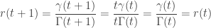
Suppose γ is another function satisfying (1) – (3), and consider the function

Then r is a meromorphic function with r(1) = γ(1)/Γ(1) = 1/1 = 1 and

Conversely, if r is any singly-periodic meromorphic function with period 1 and r(1) = 1, and we let γ(t) := r(t) Γ(t), then γ clearly satisfies (1) – (3).  So, given that we already know about the classical Γ function, the problem of classifying every function satisfying (1) – (3) reduces to the problem of classifying these functions r.

Taking the quotient of the complex plane by the translation sending z to z+1 gives us a cylinder, so equivalently we’re looking for meromorphic functions on this cylinder.  This cylinder is isomorphic (a.k.a. biholomorphic, a.k.a. conformally equivalent) to the punctured complex plane.

Unfortunately the noncompactness of the cylinder is a serious problem if we want to describe its function field.  I’m not an expert here, but my understanding is that the situation looks like this:

• The holomorphic periodic functions on the cylinder are just given by Fourier series.
• The meromorphic ones with finitely many poles are just ratios of the holomorphic ones.
• The meromorphic ones with infinitely many poles, though, aren’t so easy to describe.

One way people try to deal with this situation is by putting some arbitrary analytic condition on the functions that limits exposure to the third class of functions.  This is in essence what the Wielandt characterization of the Gamma function is doing.

For more on the function field of the cylinder, see:

• Elliptic functions and (meromorphic) simply periodic functions on math.SE

---

*It’s probably worth saying a couple of things for people who aren’t familiar with the subject.  These are the sorts of things that bothered me when I was first learning complex analysis and which, while sort of appearing in texts, never seem to be highlighted to the extent that they deserve.

First, notice that if we try to plug in t=0 into this functional equation, we get

1 = γ(1) = 0 γ(0),

which we cannot solve for γ(0).  So what do we mean when we say that γ satisfies this functional equation?  Well, we mean that it’s satisfied whenever both t and t+1 are in the domain of γ.  We see in particular that t=0 cannot be in the domain of any function γ satisfying conditions (1)-(3).

This appears at first to open another can of worms, since if we’re allowed to throw points out of the domain of γ at will we could simply look at every pair of points not satisfying the functional equation and throw out one or the other of them at random.

But we’re considering a meromorphic function on the plane.  Such a function is defined at every point in the plane, minus some countable discrete set.  (“Countable” is redundant here — every uncountable set of points in the plane fails to be discrete.)  In fact, by the Riemann removable singularities theorem, we can further insist that such a function is only undefined where it “has to be” (i.e., where the function approaches infinity in magnitude near a point).  To be quite technical, we generally think not of a particular meromorphic function but rather of an equivalence classes of meromorphic functions under the relation f~g if f(z) = g(z) at every point z in the domain of both functions.

Anyway, the point is that everything’s fine — we won’t have any analytic pathologies creeping in.

Inner product spaces, I – Real closed fields

I’ve always felt sort of uneasy about the way linear algebra is presented: you start off doing all this stuff that makes complete sense, and works over arbitrary fields, and then suddenly you’re doing something with all these complex conjugates and conjugate transposes and real symmetric matrices and so forth and nothing makes sense any more.  So I’m going to try to say something about that here.

Everything in the theory of inner products is based on three properties that look simple enough at first glance, but appear more and more bizarre as you consider them more deeply:

• The real numbers are an ordered field.
• The real numbers aren’t algebraically closed, but their algebraic closure (the complex numbers) forms a degree-2 extension.
• The norm of a nonzero complex number is a positive real number.

(By the way, what do we mean by the norm here?  Well, it’s probably exactly what you think, namely

.

But the norm is something more general: if we have a finite Galois extension , then we can define a function by

 Since consists of the identity and complex conjugation, we recover

.)

The fact that  for is specific to $latex \mathbb{C}/\mathbb{R}$; for instance, if is some squarefree positive integer, then we have

Anyway, here’s why this is all pretty weird:

• For almost any other field, the algebraic closure is an infinite-dimensional extension, so we have no hope of getting a norm map like this.  In fact, if we have a field whose algebraic closure is a finite-dimensional extension, then  is a real closed field, meaning that it looks very much like the real numbers, and moreover .  (This is the Artin-Schreier theorem.)
• In particular, if is an ordered field then for .
• So, there seem to be two completely separate kinds of non-algebraically closed fields: those that behave exactly like this (such as the real algebraic numbers, reals, and the field of real Puiseux series), and those that behave nothing like this but much like one another (such as the rational numbers, number fields in general, positive characteristic fields, etc.).

The fact that we have (1) an ordered field R (2) whose algebraic closure C is a finite-degree extension  such that (3) for nonzero allows us to extend the theory of linear algebra (over both R and C!) in some strange new directions.

A more motivated proof of the Pythagorean theorem

So far every proof I’ve known of the Pythagorean theorem has adhered to a narrative along the lines of

• Notice, purely by accident, that in known right triangles it appears that the square on the hypotenuse is always equal to the sum of the squares on the other two sides.
• Conjecture that this holds in general.
• Draw a right triangle and a square on each side.
• Figure out some ingenious geometric decomposition reassembling the two smaller squares into a copy of the bigger one.

This is fairly unsatisfying, because it only tells us that the theorem is true; it doesn’t do much to tell us why it’s true, or give us much intuition for what kind of information it does or does not encode.

Today I wondered if there was a better explanation, and I came across this:

Pythagoras’s theorem | What’s New

Terry Tao writes:

it is perhaps the most intuitive proof of the theorem that I have seen yet

The proof just comes down to examining the (obviously useful) construction where a right triangle is split into two smaller right triangles, both of which are similar to the big one.

The Weyl Group of GL(n, C)

Here’s a cleaner explanation of the Weyl group of GL(n) than I’ve seen before.  I came up with this myself, but it’s straightforward enough that I’m sure I’m not the first.

Let V be an n-dimensional complex vector space, and fix a basis for V.  Write .  Let T < G denote the subgroup of matrices which are diagonal in the basis ; this is a maximal torus.  We know that the Weyl group is isomorphic to N(T)/T, so let’s determine N(T).

Pick a matrix all of whose eigenvalues are distinct, and suppose .  Then is diagonal.  This means that A represents a change of basis from to some basis in which D is diagonal.  Now D is diagonal in some basis iff that basis consists of eigenvectors of D.  Since D was chosen in such a way that its eigenspaces are one-dimensional, the only eigenvectors of D are nonzero scalar multiples of the .  Therefore we have A = P C, where P is a permutation matrix and C is diagonal.  Conversely, it’s easy to see that any such matrix normalizes T.  

From here it’s clear that , since the cosets correspond to permutation matrices.